Gaussian Processes Barycentres

Download this notebook: barycentres.ipynb

In this notebook we’ll give an implementation of Mallasto and Feragen [2017]. In this work, the existence of a Wasserstein barycentre between a collection of Gaussian processes is proven. When faced with trying to average a set of probability distributions, the Wasserstein barycentre is an attractive choice as it enables uncertainty amongst the individual distributions to be incorporated into the averaged distribution. When compared to a naive mean of means and mean of variances approach to computing the average probability distributions, it can be seen that Wasserstein barycentres offer significantly more favourable uncertainty estimation.

import typing as tp

from utils import use_mpl_style
import jax

# Enable Float64 for more stable matrix inversions.
from jax import config
import jax.numpy as jnp
import jax.random as jr
import jax.scipy.linalg as jsl
from jaxtyping import install_import_hook
import matplotlib.pyplot as plt
try:
    from myst_nb import glue
except ImportError:  # notebook downloaded and run outside the docs build
    def glue(*args, **kwargs):
        """No-op stand-in: gluing only matters when Sphinx renders this page."""
import numpyro.distributions as npd

config.update("jax_enable_x64", True)


with install_import_hook("gpjax", "beartype.beartype"):
    import gpjax as gpx


key = jr.key(123)

# set the default style for plotting
use_mpl_style()

cols = plt.rcParams["axes.prop_cycle"].by_key()["color"]

Background

Wasserstein distance

The 2-Wasserstein distance metric between two probability measures \(\mu\) and \(\nu\) quantifies the minimal cost required to transport the unit mass from \(\mu\) to \(\nu\), or vice-versa. Typically, computing this metric requires solving a linear program. However, when \(\mu\) and \(\nu\) both belong to the family of multivariate Gaussian distributions, the solution is analytically given by

(1)\[\begin{split} \begin{aligned} W_2^2(\mu, \nu) & = \lVert m_1- m_2 \rVert^2_2 \\ & \quad + \operatorname{Tr}(S_1 + S_2 - 2(S_1^{1/2}S_2S_1^{1/2})^{1/2}), \end{aligned} \end{split}\]

where \(\mu \sim \mathcal{N}(m_1, S_1)\) and \(\nu\sim\mathcal{N}(m_2, S_2)\).

Wasserstein barycentre

For a collection of \(T\) measures \(\lbrace\mu_i\rbrace_{t=1}^T \in \mathcal{P}_2(\theta)\), the Wasserstein barycentre \(\bar{\mu}\) is the measure that minimises the average Wasserstein distance to all other measures in the set. More formally, the Wasserstein barycentre is the Fréchet mean on a Wasserstein space that we can write as

(2)\[ \bar{\mu} = \operatorname{argmin}_{\mu\in\mathcal{P}_2(\theta)}\sum_{t=1}^T \alpha_t W_2^2(\mu, \mu_t), \]

where \(\alpha\in\mathbb{R}^T\) is a weight vector that sums to 1.

As with the Wasserstein distance, identifying the Wasserstein barycentre \(\bar{\mu}\) is often an computationally demanding optimisation problem. However, when all the measures admit a multivariate Gaussian density, the barycentre \(\bar{\mu} = \mathcal{N}(\bar{m}, \bar{S})\) has analytical solutions

(3)\[\begin{split} \begin{aligned} \bar{m} & = \sum_{t=1}^T \alpha_t m_t\,, \\ \bar{S} & = \sum_{t=1}^T\alpha_t (\bar{S}^{1/2}S_t\bar{S}^{1/2})^{1/2}\,. \end{aligned} \end{split}\]

Identifying \(\bar{S}\) is achieved through a fixed-point iterative update.

Barycentre of Gaussian processes

It was shown in Mallasto and Feragen [2017] that the barycentre \(\bar{f}\) of a collection of Gaussian processes \(\lbrace f_i\rbrace_{i=1}^T\) such that \(f_i \sim \mathcal{GP}(m_i, K_i)\) can be found using the same solutions as in Eq. 3. For a full theoretical understanding, we recommend reading the original paper. However, the central argument to this result is that one can first show that the barycentre GP \(\bar{f}\sim\mathcal{GP}(\bar{m}, \bar{S})\) is non-degenerate for any finite set of GPs \(\lbrace f_t\rbrace_{t=1}^T\) i.e., \(T<\infty\). With this established, one can show that for a \(n\)-dimensional finite Gaussian distribution \(f_{i,n}\), the Wasserstein metric between any two Gaussian distributions \(f_{i, n}, f_{j, n}\) converges to the Wasserstein metric between GPs as \(n\to\infty\).

In this notebook, we will demonstrate how this can be achieved in GPJax.

Dataset

We’ll simulate five datasets and develop a Gaussian process posterior before identifying the Gaussian process barycentre at a set of test points. Each dataset will be a sine function with a different vertical shift, periodicity, and quantity of noise.

n = 100
n_test = 200
n_datasets = 5

x = jnp.linspace(-5.0, 5.0, n).reshape(-1, 1)
xtest = jnp.linspace(-5.5, 5.5, n_test).reshape(-1, 1)
f = lambda x, a, b: a + jnp.sin(b * x)

ys = []
for _ in range(n_datasets):
    key, subkey = jr.split(key)
    vertical_shift = jr.uniform(subkey, minval=0.0, maxval=2.0)
    period = jr.uniform(subkey, minval=0.75, maxval=1.25)
    noise_amount = jr.uniform(subkey, minval=0.01, maxval=0.5)
    noise = jr.normal(subkey, shape=x.shape) * noise_amount
    ys.append(f(x, vertical_shift, period) + noise)

y = jnp.hstack(ys)

fig, ax = plt.subplots()
ax.plot(x, y, "x")
plt.show()

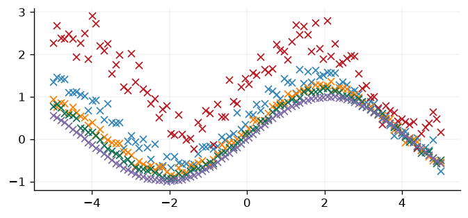
Fig. 25 The five simulated datasets, each a sine function with its own vertical shift, periodicity and noise level.

Learning a posterior distribution

We’ll now independently learn Gaussian process posterior distributions for each of the datasets in Fig. 25. Each fit returns a GaussianDistribution, and it is the mean vector and covariance matrix of these that the barycentre is computed from below. We won’t spend any time here discussing how GP hyperparameters are optimised. For advice on achieving this, see the Regression notebook for advice on optimisation and the Kernels notebook for advice on selecting an appropriate kernel.

def fit_gp(x: jax.Array, y: jax.Array) -> gpx.distributions.GaussianDistribution:
    if y.ndim == 1:
        y = y.reshape(-1, 1)
    D = gpx.Dataset(X=x, y=y)

    likelihood = gpx.likelihoods.Gaussian()
    posterior = (
        gpx.gps.Prior(
            mean_function=gpx.mean_functions.Constant(), kernel=gpx.kernels.RBF()
        )
        * likelihood
    )

    nmll = lambda p, d: -gpx.objectives.conjugate_mll(p, d)
    opt_posterior, _ = gpx.fit_scipy(
        model=posterior,
        objective=nmll,
        train_data=D,
    )
    latent_dist = opt_posterior.predict(xtest, train_data=D)
    return opt_posterior.likelihood(latent_dist)


posterior_preds = [fit_gp(x, i) for i in ys]

Optimization terminated successfully.
         Current function value: -31.899723
         Iterations: 12
         Function evaluations: 18
         Gradient evaluations: 18
Optimization terminated successfully.
         Current function value: 28.634760
         Iterations: 11
         Function evaluations: 20
         Gradient evaluations: 20
Optimization terminated successfully.
         Current function value: -102.556037
         Iterations: 10
         Function evaluations: 19
         Gradient evaluations: 19
Optimization terminated successfully.
         Current function value: -143.067418
         Iterations: 13
         Function evaluations: 23
         Gradient evaluations: 23
Optimization terminated successfully.
         Current function value: -271.634988
         Iterations: 11
         Function evaluations: 17
         Gradient evaluations: 17

Computing the barycentre

In GPJax, the predictive distribution of a GP is given by a TensorFlow Probability distribution, making it straightforward to extract the mean vector and covariance matrix of each GP for learning a barycentre. We implement the fixed point scheme given in Eq. 3 in the following cell by utilising Jax’s vmap operator to speed up large matrix operations using broadcasting in tensordot.

def sqrtm(A: jax.Array):
    return jnp.real(jsl.sqrtm(A))


def wasserstein_barycentres(
    distributions: list[gpx.distributions.GaussianDistribution], weights: jax.Array
):
    covariances = [d.covariance_matrix for d in distributions]
    cov_stack = jnp.stack(covariances)
    stack_sqrt = jax.vmap(sqrtm)(cov_stack)

    def step(covariance_candidate: jax.Array, idx: None):
        inner_term = jax.vmap(sqrtm)(
            jnp.matmul(jnp.matmul(stack_sqrt, covariance_candidate), stack_sqrt)
        )
        fixed_point = jnp.tensordot(weights, inner_term, axes=1)
        return fixed_point, fixed_point

    return step

With a function defined for learning a barycentre, we’ll now compute it using the lax.scan operator that drastically speeds up for loops in Jax (see the Jax documentation). The iterative update will be executed 50 times, with convergence measured by the difference between the previous and current iteration that we can confirm by inspecting the sequence array in the following cell.

weights = jnp.ones((n_datasets,)) / n_datasets

means = jnp.stack([d.mean for d in posterior_preds])
barycentre_mean = jnp.tensordot(weights, means, axes=1)

step_fn = jax.jit(wasserstein_barycentres(posterior_preds, weights))
initial_covariance = jnp.eye(n_test)

barycentre_covariance, sequence = jax.lax.scan(
    step_fn, initial_covariance, jnp.arange(50)
)
glue("barycentres-num-iterations", f"{sequence.shape[0]}", display=False)
L = jnp.linalg.cholesky(barycentre_covariance)

barycentre_process = npd.MultivariateNormal(barycentre_mean, scale_tril=L)

Plotting the result

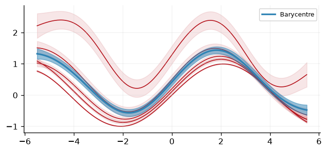
With a barycentre learned, we can visualise the result. We can see that the result looks reasonable as it follows the sinusoidal curve of all the inferred GPs, and the uncertainty bands are sensible.

def plot(
    dist: npd.MultivariateNormal | gpx.distributions.GaussianDistribution,
    ax,
    color: str,
    label: str = None,
    ci_alpha: float = 0.2,
    linewidth: float = 1.0,
    zorder: int = 0,
):
    mu = dist.mean
    sigma = jnp.sqrt(dist.variance)
    ax.plot(xtest, mu, linewidth=linewidth, color=color, label=label, zorder=zorder)
    ax.fill_between(
        xtest.squeeze(),
        mu - sigma,
        mu + sigma,
        alpha=ci_alpha,
        color=color,
        zorder=zorder,
    )


fig, ax = plt.subplots()
[plot(d, ax, color=cols[1], ci_alpha=0.1) for d in posterior_preds]
plot(
    barycentre_process,
    ax,
    color=cols[0],
    label="Barycentre",
    ci_alpha=0.5,
    linewidth=2,
    zorder=1,
)
ax.legend()

<matplotlib.legend.Legend at 0x7fcfd5d02c50>

Displacement interpolation

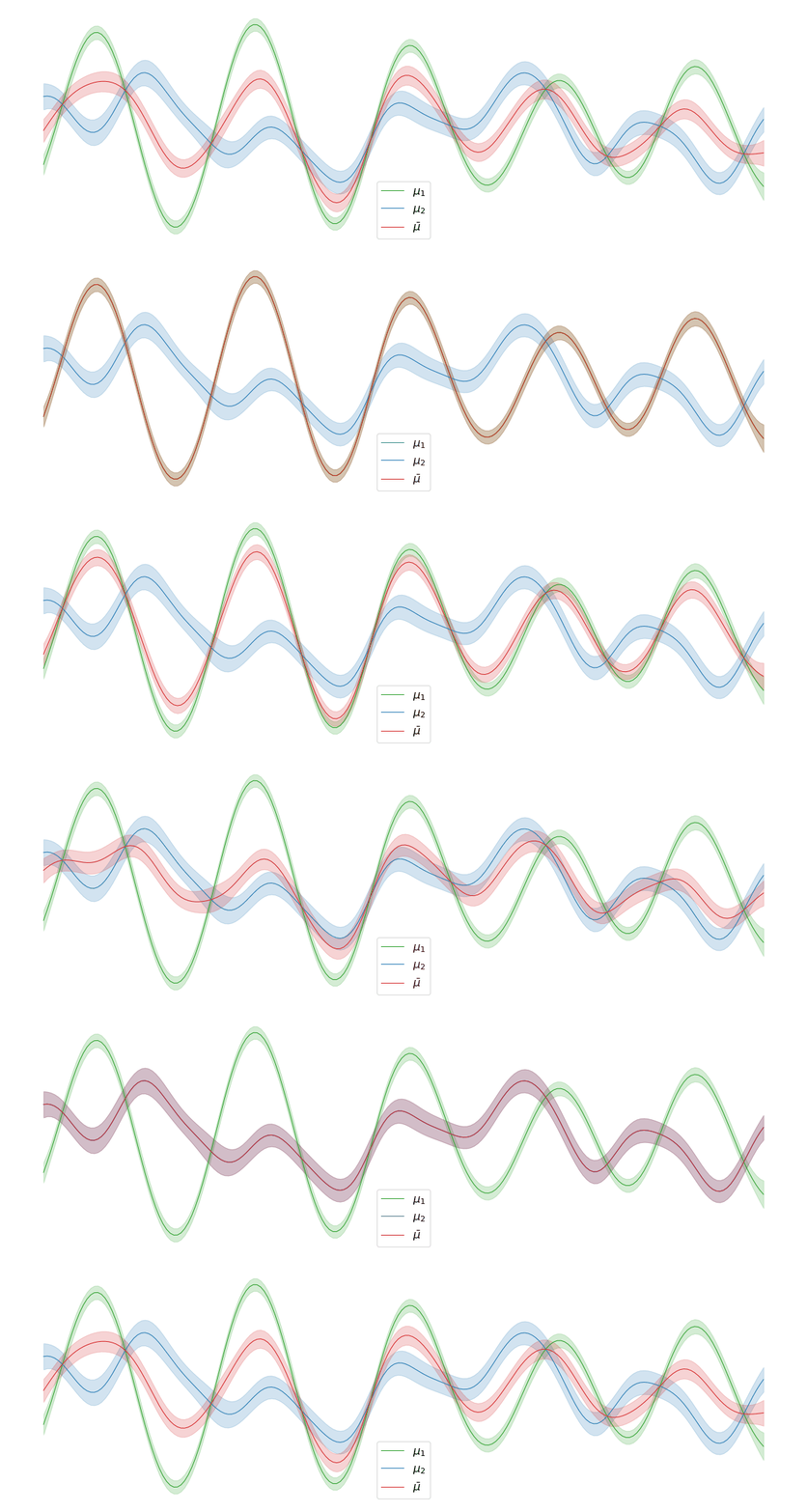
In the above example, we assigned uniform weights to each of the posteriors within the barycentre. In practice, we may have prior knowledge of which posterior is most likely to be the correct one. Regardless of the weights chosen, the barycentre remains a Gaussian process. We can interpolate between a pair of posterior distributions \(\mu_1\) and \(\mu_2\) to visualise the corresponding barycentre \(\bar{\mu}\).

System configuration

%reload_ext watermark
%watermark -n -u -v -iv -w -a 'Thomas Pinder'

Author: Thomas Pinder

Last updated: Fri, 07 Aug 2026

Python implementation: CPython
Python version       : 3.11.15
IPython version      : 9.15.0

gpjax     : 0.18.0
jax       : 0.10.2
jaxtyping : 0.3.11
matplotlib: 3.11.1
myst_nb   : 1.4.0
numpyro   : 0.21.0

Watermark: 2.6.0