Regression

Download this notebook: regression.ipynb

In this notebook we demonstrate how to fit a Gaussian process regression model. We move quickly through the theory; if any of it is unfamiliar, our introduction to Gaussian processes derives the same model from Bayes’ theorem.

# Enable Float64 for more stable matrix inversions.
from utils import (
    use_mpl_style,
)
from jax import config
import jax.numpy as jnp
import jax.random as jr
from jaxtyping import install_import_hook
import matplotlib as mpl
import matplotlib.pyplot as plt

from utils import use_mpl_style, clean_legend

config.update("jax_enable_x64", True)


with install_import_hook("gpjax", "beartype.beartype"):
    import gpjax as gpx


key = jr.key(123)

# set the default style for plotting
use_mpl_style()

cols = mpl.rcParams["axes.prop_cycle"].by_key()["color"]

Dataset

With the necessary modules imported, we simulate a dataset \(\mathcal{D} = (\boldsymbol{x}, \boldsymbol{y}) = \{(x_i, y_i)\}_{i=1}^{100}\) with inputs \(\boldsymbol{x}\) sampled uniformly on \((-3., 3)\) and corresponding independent noisy outputs

(1)\[ \boldsymbol{y} \sim \mathcal{N} \left(\sin(4\boldsymbol{x}) + \cos(2 \boldsymbol{x}), \textbf{I} * 0.3^2 \right). \]

We store our data \(\mathcal{D}\) as a GPJax Dataset and create test inputs and labels for later.

n = 100
noise = 0.3

key, subkey = jr.split(key)
x = jr.uniform(key=key, minval=-3.0, maxval=3.0, shape=(n,)).reshape(-1, 1)
f = lambda x: jnp.sin(4 * x) + jnp.cos(2 * x)
signal = f(x)
y = signal + jr.normal(subkey, shape=signal.shape) * noise

D = gpx.Dataset(X=x, y=y)

xtest = jnp.linspace(-3.5, 3.5, 500).reshape(-1, 1)
ytest = f(xtest)

To better understand what we have simulated, we plot both the underlying latent function and the observed data that is subject to Gaussian noise.

fig, ax = plt.subplots()
ax.plot(x, y, "o", label="Observations", color=cols[0])
ax.plot(xtest, ytest, label="Latent function", color=cols[1])
ax.legend(loc="best")
plt.show()

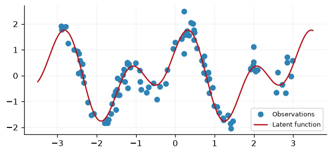
Fig. 4 The simulated dataset: 100 noisy observations scattered around the latent function that generated them.

Our aim in this tutorial will be to reconstruct the latent function from our noisy observations \(\mathcal{D}\) via Gaussian process regression. We begin by defining a Gaussian process prior in the next section.

Defining the prior

A zero-mean Gaussian process (GP) places a prior distribution over real-valued functions \(f(\cdot)\) where \(f(\boldsymbol{x}) \sim \mathcal{N}(0, \mathbf{K}_{\boldsymbol{x}\boldsymbol{x}})\) for any finite collection of inputs \(\boldsymbol{x}\).

Here \(\mathbf{K}_{\boldsymbol{x}\boldsymbol{x}}\) is the Gram matrix generated by a user-specified symmetric, non-negative definite kernel function \(k(\cdot, \cdot')\) with \([\mathbf{K}_{\boldsymbol{x}\boldsymbol{x}}]_{i, j} = k(x_i, x_j)\). The choice of kernel function is critical as, among other things, it governs the smoothness of the outputs that our GP can generate. Our introduction to kernels works through what each kernel assumes and how to pick between them.

For simplicity, we consider a radial basis function (RBF) kernel:

(2)\[ k(x, x') = \sigma^2 \exp\left(-\frac{\lVert x - x' \rVert_2^2}{2 \ell^2}\right). \]

On paper a GP is written as \(f(\cdot) \sim \mathcal{GP}(\textbf{0}, k(\cdot, \cdot'))\), we can reciprocate this process in GPJax via defining a Prior with our chosen RBF kernel.

kernel = gpx.kernels.RBF()  # 1-dimensional input
meanf = gpx.mean_functions.Zero()
prior = gpx.gps.Prior(mean_function=meanf, kernel=kernel)

The above construction forms the foundation for GPJax’s models. Moreover, the GP prior we have just defined can be represented by a TensorFlow Probability multivariate Gaussian distribution. Such functionality enables trivial sampling, and the evaluation of the GP’s mean and covariance.

Since we want to sample from the full posterior, we need to calculate the full covariance matrix. We can enforce this by including the covariance = "dense" attribute when predicting. Note this is what will be defaulted if left blank.

prior_dist = prior.predict(xtest, covariance="dense")

prior_mean = prior_dist.mean
prior_std = prior_dist.variance
samples = prior_dist.sample(key=key, sample_shape=(20,))


fig, ax = plt.subplots()
ax.plot(xtest, samples.T, alpha=0.5, color=cols[0], label="Prior samples")
ax.plot(xtest, prior_mean, color=cols[1], label="Prior mean")
ax.fill_between(
    xtest.flatten(),
    prior_mean - prior_std,
    prior_mean + prior_std,
    alpha=0.3,
    color=cols[1],
    label="Prior variance",
)
ax.legend(loc="best")
clean_legend(ax)
plt.show()

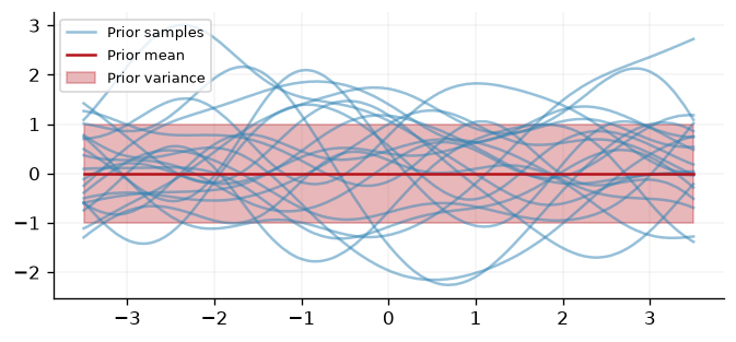
Fig. 5 Twenty function samples drawn from the zero-mean RBF prior, shown alongside the prior mean and variance band.

Constructing the posterior

Having defined our GP, we proceed to define a description of our data \(\mathcal{D}\) conditional on our knowledge of \(f(\cdot)\) - this is exactly the notion of a likelihood function \(p(\mathcal{D} | f(\cdot))\). Whilst the choice of likelihood is a critical in Bayesian modelling, for simplicity we consider a Gaussian with noise parameter \(\alpha\)

(3)\[ p(\mathcal{D} | f(\cdot)) = \mathcal{N}(\boldsymbol{y}; f(\boldsymbol{x}), \textbf{I} \alpha^2). \]

This is defined in GPJax through calling a Gaussian instance. The likelihood guide covers the other likelihoods GPJax provides and what each one assumes about the observations.

likelihood = gpx.likelihoods.Gaussian()

The prior and likelihood together define the joint model over the latent function and the observations,

(4)\[ p(f(\cdot), \mathcal{D}) = p(\mathcal{D} | f(\cdot))\, p(f(\cdot)). \]

Mimicking this equation, the joint model is established in GPJax through the * operator. Conditioning it on the data — model.condition(D), or the operator form model | D that reads as \(p(f \mid \mathcal{D})\) — yields the posterior process.

model = prior * likelihood

Parameter state

As outlined in the PyTrees documentation, parameters are contained within the model and for the leaves of the PyTree. Consequently, in this particular model, we have three parameters: the kernel lengthscale, kernel variance and the observation noise variance. Whilst we have initialised each of these to 1, we can learn Type 2 MLEs for each of these parameters by optimising the marginal log-likelihood (MLL).

print(-gpx.objectives.conjugate_mll(model, D))

132.6462594200374

We can now define an optimiser. For this example we’ll use the bfgs optimiser.

opt_model, history = gpx.fit_scipy(
    model=model,
    objective=lambda p, d: -gpx.objectives.conjugate_mll(p, d),
    train_data=D,
)

print(-gpx.objectives.conjugate_mll(opt_model, D))

Optimization terminated successfully.
         Current function value: 55.469226
         Iterations: 12
         Function evaluations: 19
         Gradient evaluations: 19
55.46922647118372

To inspect the learned hyperparameters, we can render a summary table of the optimised posterior with gpx.summarise. This shows each parameter’s constrained value, its bijector, and whether it is trainable — a quick sanity check after optimisation.

gpx.summarise(opt_model)

ConjugateModel                                                                                           
╭──────────────────────────────┬─────────────────┬───────┬──────────┬───────┬───────────┬───────┬───────╮
│ Parameter                    │ Class           │ Value │ Bijector │ Prior │ Trainable │ Shape │ Dtype │
├──────────────────────────────┼─────────────────┼───────┼──────────┼───────┼───────────┼───────┼───────┤
│ prior.kernel.lengthscale     │ PositiveReal    │ 0.47  │ Softplus │ -     │ yes       │ ()    │ f64   │
│ prior.kernel.variance        │ NonNegativeReal │ 1.69  │ Softplus │ -     │ yes       │ ()    │ f64   │
│ prior.mean_function.constant │ Array           │ 0     │ Identity │ -     │ no        │ ()    │ f64   │
│ likelihood.obs_stddev        │ NonNegativeReal │ 0.318 │ Softplus │ -     │ yes       │ ()    │ f64   │
╰──────────────────────────────┴─────────────────┴───────┴──────────┴───────┴───────────┴───────┴───────╯
4 parameters, 3 trainable                                                                                

Prediction

Equipped with the posterior and a set of optimised hyperparameter values, we are now in a position to query our GP’s predictive distribution at novel test inputs. To do this, we condition the optimised model on the training data — this factorises the training covariance exactly once and caches it — and then query the resulting posterior process at the test inputs. Pushing the latent distribution through the likelihood yields the predictive distribution, upon which mean and stddev can be used to extract the predictive mean and standard deviation.

We are only concerned here with the variance at the test points themselves, so we request the diagonal covariance via covariance="diagonal".

posterior = opt_model.condition(D)  # equivalently: opt_model | D
latent_dist = posterior(xtest, covariance="diagonal")
predictive_dist = opt_model.likelihood(latent_dist)

predictive_mean = predictive_dist.mean
predictive_std = jnp.sqrt(predictive_dist.variance)

With the predictions and their uncertainty acquired, we illustrate the GP’s performance at explaining the data \(\mathcal{D}\) and recovering the underlying latent function of interest.

fig, ax = plt.subplots(figsize=(7.5, 2.5))
ax.plot(x, y, "x", label="Observations", color=cols[0], alpha=0.5)
ax.fill_between(
    xtest.squeeze(),
    predictive_mean - 2 * predictive_std,
    predictive_mean + 2 * predictive_std,
    alpha=0.2,
    label="Two sigma",
    color=cols[1],
)
ax.plot(
    xtest,
    predictive_mean - 2 * predictive_std,
    linestyle="--",
    linewidth=1,
    color=cols[1],
)
ax.plot(
    xtest,
    predictive_mean + 2 * predictive_std,
    linestyle="--",
    linewidth=1,
    color=cols[1],
)
ax.plot(
    xtest, ytest, label="Latent function", color=cols[0], linestyle="--", linewidth=2
)
ax.plot(xtest, predictive_mean, label="Predictive mean", color=cols[1])
ax.legend(loc="center left", bbox_to_anchor=(0.975, 0.5))
plt.show()

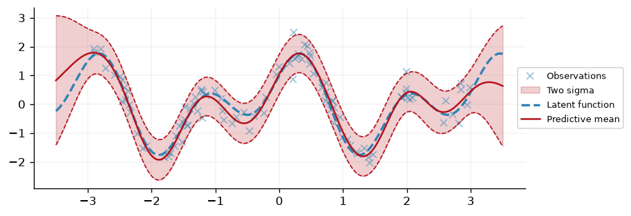
Fig. 6 The optimised posterior predictive mean and its two-sigma band, plotted against the observations and the true latent function.

System configuration

%reload_ext watermark
%watermark -n -u -v -iv -w -a 'Thomas Pinder & Daniel Dodd'

Author: Thomas Pinder & Daniel Dodd

Last updated: Fri, 07 Aug 2026

Python implementation: CPython
Python version       : 3.11.15
IPython version      : 9.15.0

gpjax     : 0.18.0
jax       : 0.10.2
jaxtyping : 0.3.11
matplotlib: 3.11.1

Watermark: 2.6.0